This task shows how to analyze the distance between any two geometric elements, or between two sets of elements.
This command is only available with:
-
FreeStyle Shaper
-
Wireframe and Surface for Building 1.
-
When computing the distance between two curves, there is no negative values possible as opposed to when analyzing the distance between a surface and another element. Indeed, surfaces present an orientation in all three space directions whereas, in the case of planar curves for example, only two directions are defined. Therefore the distance is always expressed with a positive value when analyzing the distance between two curves.
-
The element whose dimension is the smallest (0 for points,1 for curves, 2 for surfaces for example) is automatically discretized, if needed.
When selecting a set of elements, the system compares the greatest dimension of all elements in each set, and discretizes the one with the smallest dimension. -
When the computed distance between two elements is less than the model resolution or any of the following:
-
0.001mm in Standard scale,
-
0.1mm in Large scale,
-
0.01 µm in Small scale,
then the Distance Analysis displays zero value for the computed distance. The precision is not guaranteed for computed distance values less than the model precision.
-
Open the FreeStyle_Part_11.CATPart document.
-
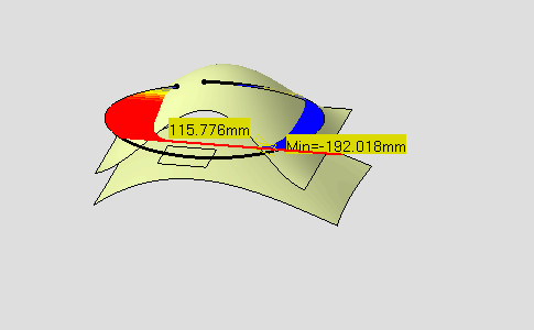
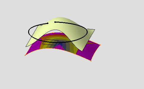
Select Curve.1.
The Distance dialog box appears, the Second set state is selected:

The Distance dialog box displays the following options:
-
Selection State: Defines the elements to be analyzed. To add or remove an element in a set, use the Ctrl key.
-
First set: Defines the first set of elements to be analyzed.
All the elements selected before running the command are considered in the First set, the Second set is then automatically selected. -
Second set: Defines the second set of elements to be analyzed.
-
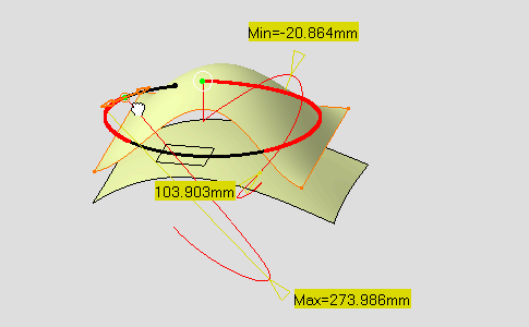
Running point: Allows you to display more precise distance value between the point below the pointer and the other set of elements when you move the pointer over the discretized element.
The projection is visualized and the value is displayed in the geometry area. Note that the analyzed point is not necessarily a discretized point in this case. This is obvious when a low discretization value is set, as shown here.
-
-
Invert Analysis: Inverts the computation direction. In some cases, when inverting the computation direction does not make sense, when one of the elements is a plane for example, the Invert Analysis button is grayed.
-
Projection Space: Defines the preprocessing of the input elements used for the computation.
-
 No Projection Of Elements: Elements are not modified and the computation is done
between the initial elements.
No Projection Of Elements: Elements are not modified and the computation is done
between the initial elements. -
 Projection in X direction: Projection
according to the X-axis, the computation is done between the projection
of selected elements. Only available when analyzing distances between
curves.
Projection in X direction: Projection
according to the X-axis, the computation is done between the projection
of selected elements. Only available when analyzing distances between
curves. -
 Projection in Y direction: Projection
according to the Y-axis, the computation is done between the projection
of selected elements. Only available when analyzing distances between
curves.
Projection in Y direction: Projection
according to the Y-axis, the computation is done between the projection
of selected elements. Only available when analyzing distances between
curves. -
 Projection in Z direction: Projection
according to the Z-axis, the computation is done between the projection
of selected elements. Only available when analyzing distances between
curves.
Projection in Z direction: Projection
according to the Z-axis, the computation is done between the projection
of selected elements. Only available when analyzing distances between
curves. -
 Projection in compass direction:
Projection according to the compass current orientation, the
computation is done between the projection of selected elements.
Projection in compass direction:
Projection according to the compass current orientation, the
computation is done between the projection of selected elements. -
 Planar
distance: The distance is computed between a curve and the
intersection of the plane containing that curve. Available only when
analyzing distances between a curve and a plane.
Planar
distance: The distance is computed between a curve and the
intersection of the plane containing that curve. Available only when
analyzing distances between a curve and a plane.
-
-
Measurement Direction: Provides options to define how set the direction used for the distance computation.
-
 Normal
distance: The distance is computed according to the normal to
the other set of elements.
Normal
distance: The distance is computed according to the normal to
the other set of elements. -
Distance in X direction: The
distance is computed according to the X-axis.
-
Distance in Y direction: The
distance is computed according to the Y-axis.
-
Distance in Z direction: The
distance is computed according to the Z-axis
-
Distance in compass direction:
The distance is computed according to the compass orientation.
-
-
Display Options: Defines the display options.
-
 2D
Diagram: Displays a 2D diagram representing the distance
variation
2D
Diagram: Displays a 2D diagram representing the distance
variation -
 Full color
range: Makes a complete analysis based on the chosen color range.
This allows you to see exactly how the evolution of the distance is
performed on the selected element, this functionality is P2-only.
Full color
range: Makes a complete analysis based on the chosen color range.
This allows you to see exactly how the evolution of the distance is
performed on the selected element, this functionality is P2-only. -
 Limited
color range: Makes a simplified analysis, with only three values
and four colors, display by default.
Limited
color range: Makes a simplified analysis, with only three values
and four colors, display by default.
-
-
Click the More button in the Distance dialog box.
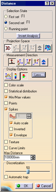
The Distance dialog box displays the following extended options:
-
Color scale: Displays the Distance.x dialog box with the full or the limited color range.
-
Statistical distribution: Displays the percentage of points between two values, effective when the Color scale option is selected.
-
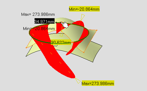
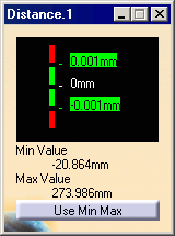
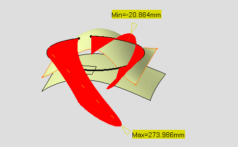
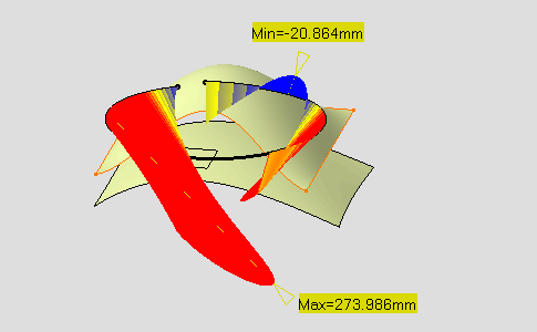
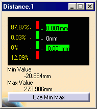
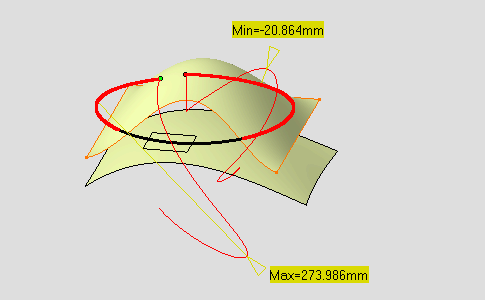
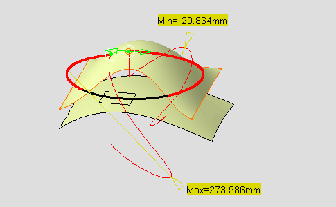
Min/Max values: Displays the minimum and maximum distance values and locations on the geometry.
-
Points: Displays the distance analysis in the shape of points only on the geometry.
-
Spikes: Displays the distance analysis in the shape of spikes on the geometry.
You can further choose to:-
 Sets the ratio
for the spike size, available only when the Auto scale
option is cleared.
Sets the ratio
for the spike size, available only when the Auto scale
option is cleared. -
Auto scale: Sets an automatic optimized spike size.
-
Inverted: Inverts the spike visualization on the geometry
-
Envelope: Displays the envelope, that is the curve connecting all spikes together
-
-
Texture: Checks the analysis using color distribution:
-
This option is only available with surface elements in at least one set, providing this set is discretized.
-
The distance is computed from this discretized set to the other set.
-
The texture mapping is computed on the discretized surface. It is not advised to use it with planar surfaces or ruled surfaces.
-
A user defined color without associated value is added in the full or the limited color range, which allows you to manage an independent color for no valuated area.
-
-
Statistical distribution, Min/Max values, and Points cannot be visualized when using the Texture option.
-
The discretization option should be set to a maximum (in Infrastructure User's Guide, see Improving Performances, the 3D Accuracy > Fixed option should be set to 0.01).
-
Run the View > Render Style > Customize View command, and select in the View Mode Customization dialog box which appears the following options to be able to see the analysis results on the selected element. Otherwise a warning is issued:
-
Select the Edges and points option then the All edges option.
-
Select the Shading option then the Material option.
-
-
Curve Limits: Re-limits the discretized curve, this functionality is P2-only.
-
Max Distance: Re-limits the maximal distance value.
-
Discretization: Reduces or increases the number of points of discretization from the set of elements which are taken into account when computing the distance.
-
Automatic trap: delimits the set of points of discretization to be taken into account for the computation, in the case of a large set of points of discretization, thus improving the performances.
-
When using the Automatic trap option, a mean plane of the non-discretized element is computed.
If points of discretization are too scattered according to this mean plane, this option may not be able to take into account as many points as needed for a consistent result such as an incomplete result (some computed areas are not taken into account) or no result.
In this case, it is best to clear the option.
-
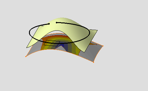
Select Surface.1.
-
Select Running Point and move the pointer over the discretized element.
-
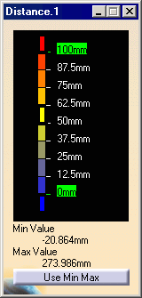
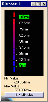
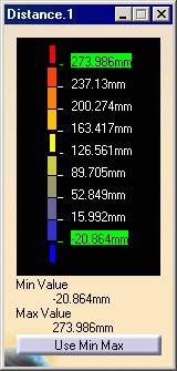
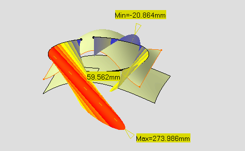
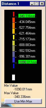
Select Color Scale option.
The Distance.1 dialog box appears and shows the Limited color range and identifies the maximum and minimum values for the analysis.
The distance analysis is computed. Each color identifies all discretization points located at a distance between two values, as defined in the Limited color range dialog box.
-
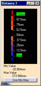
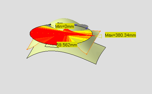
Select Full color range
.
The Distance.1 dialog box shows the Full color range and identifies the maximum and minimum values for the analysis.
The distance analysis is computed. Each color identifies all discretization points located at a distance between two values, as defined in the Full color range dialog box.
The following description is valid for the Limited color range and the Full color range dialog boxes. Whichever mode you choose the use of the color scale is identical: it lets you define colors in relation to distance values. You can define each of the values and color blocks, therefore attributing a color to all elements which distance falls into to given values.
-
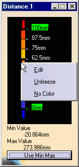
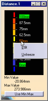
Right-click a color rectangle in the color scale to display the contextual menu:
-
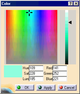
Edit contextual command allows you to modify the values in the color range to highlight specific areas of the selected surface. The Color dialog box is displayed allowing you to modify the color range.
-
Unfreeze contextual command allows you to perform a linear interpolation between non-defined colors.
-
No Color contextual command can be used to simplify the analysis, because it limits the number of displayed colors in the color scale. In this case, the selected color is hidden, and the section of the analysis on which that color was applied takes on the neighboring color.
-
-
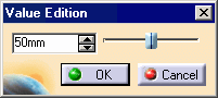
You can also right-click on the value to display the contextual menu:
-
Edit contextual command allows you to modify the edition values.
The Value Edition dialog box is displayed: enter a new value (negative values are allowed) to redefine the color scale, or use the slider to position the distance value within the allowed range, and click OK.
The value is then frozen, and displayed in a green rectangle.
-
Unfreeze contextual command allows you to perform a linear interpolation between non-defined values, meaning that between two set (or frozen) colors/values, the distribution is done progressively and evenly. This command is available for all values except for maximum and minimum values.
The unfreezed values are no longer highlighted in green. -
Use Max / Use Min contextual commands allow you to evenly distribute the color/value interpolation between the current limit values, on the top/bottom values respectively, rather than keeping it within default values that may not correspond to the scale of the geometry being analyzed. Therefore, these limit values are set at a given time, and when the geometry is modified after setting them, these limit values are not dynamically updated.
-
These commands are available for maximum and minimum values only.
-
The Use Max command is available if the maximum value is higher or equal to the medium value, otherwise you need to unfreeze the medium value first.
-
The Use Min command is available if the minimum value is lower or equal to the medium value, otherwise you need to unfreeze the medium value first.
-
-
-
Use Min Max button in the Distance Analysis.1 dialog box makes in one action the Use Max / Use Min contextual commands operation.
-
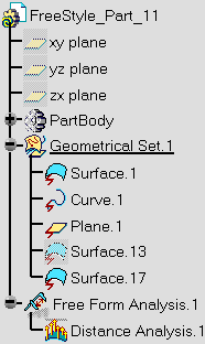
The Distance Analysis.1 is created in the specification tree under the Free Form Analysis.1
The color scale settings (colors and values) are
saved when exiting the command, meaning the same values will be set next
time you edit a given distance analysis capability.
However, new settings are available with each new distance analysis.
-
Click Use Min Max button in the Distance.1 dialog box.
Maximum and minimum values are set according to the computed values displayed below the color scale.
The color range has been redefined according to the color scale.
-
Select Planar distance
.
Distance is computed between Curve.1 and the intersection of the plane containing that curve
-
Select 3D
and the X option in
the Measurement Direction:
Distance is computed along the X direction.
-
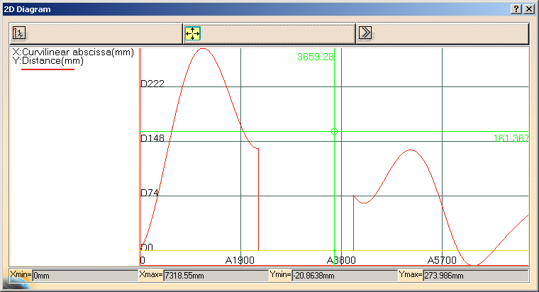
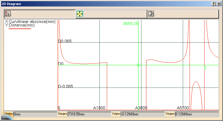
Select the Normal Direction option:
and the 2D
Diagram option:
The 2D Diagram dialog box appears and allows you to visualize the distance evolution.
The 2D Diagram dialog box displays the following options:
-
Inverse Y axis value
 :
Draws the curves in a linear horizontal
scale and and inverse vertical scale.
:
Draws the curves in a linear horizontal
scale and and inverse vertical scale.
-
Reframe
 : Reframes
the diagram within the viewer window, as you may move and zoom it within
the window.
: Reframes
the diagram within the viewer window, as you may move and zoom it within
the window. -
Display a panel with more options
 :
Displays the Diagram Options dialog box that enables you to
define more options.
:
Displays the Diagram Options dialog box that enables you to
define more options.
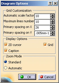
- Grid
Customization: The
number of lines
displayed on grid during
zoom depends on the
following options:
- Automatic scale factor: Defines the space between two coordinate lines when when there are not enough lines in the viewer.
- Maximum lines number: Defines the maximum number of lines displayed in the viewer without zooming.
- Primary spacing on X: Defines the distance between the coordinates of the X-axis.
- Primary spacing on Y: Defines the distance between the coordinates of the Y-axis.
- Display
Options: The
display in the 2D
Diagram can be
customized:
- 2D cursor: Select this option to display the 2D cursor.
- Caption: Select this option to display the caption area.
- Grid: Select this option to display the grid.
- Zoom
Mode: There are
two ways to zoom in the
viewer window.
- using the mouse you can navigate in the viewer graph by panning (translation) and zooming in it.
- You can define a frame in the area where to zoom in. The graphical area is selected by using trap selection with the mouse. For zoom by trap two types of stretching are available:
- Standard: There is no stretching. The area is zoomed in the window and the X-axis and Y-axis intervals depend on the values defined in Primary spacing on X and Primary spacing on Y.
- Automatic: The horizontal X-axis interval corresponds to the interval resulting from zoom. The vertical Y-axis interval corresponds to the extrema computed from the Xmin and Xmax of the X-axis interval.
The following values are displayed for all the analyzed curves in 2D Diagram dialog box:
- Xmin: The minimum abscissa of all the curves in the graphical area.
- Xmax: The maximum abscissa of all the curves in the graphical area.
- Ymin: The minimum ordinate of all the curves in the graphical area.
- Ymax: The maximum ordinate of all the curves in the graphical area.
For more information on 2D Diagram dialog box, see Performing a Curvature Analysis.
- Grid
Customization: The
number of lines
displayed on grid during
zoom depends on the
following options:
Whenever the 2D Diagram option is enabled in Distance Analysis, you can open the 2D Diagram dialog box.
-
Select the Limited color range option:
and select the
Statistical distribution option.
-
Select the Points option and clear the Spikes option.
Show the distance analysis in the shape of points only on the geometry.
-
Select the Curve Limits option.
Two manipulators appear at both extremities of the curve: they let you define new start and end points on the curve.
Start and end points are defined by a ratio of curve length between 0 and 1. If you extend the curve for instance, this ratio is kept.
-
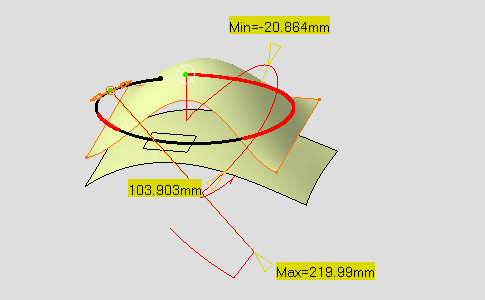
Set the Max Distance value to 220mm.
The maximum value is re-limited accordingly on the geometry.
-
Select the First set state and deselect the Curve.1 using the Ctrl key, then select Surface.17.
-
Select the Texture option, the Spikes option is automatically deselected.
-
Select Full color range
and click the
Use Min Max button in the Distance.1 dialog box.
The user defined color is displayed in the Distance.1 dialog box.
The texture mapping is displayed on Surface.17.
-
Define the color as magenta in the Distance.1 dialog box.
The non-valuated area is magenta-colored.
-
Click OK to exit the analysis while retaining it.
The analysis (identified as Distance Analysis.x) is added to the specification tree.
-
Even though you exit the analysis, the color scale is retained till you explicitly close is. This is like a shortcut allowing you to modify one of the analyzed elements, which leads to a dynamic update of the distance analysis, while viewing the set values/colors at all times and without having to edit the distance analysis.
-
When analyzing clouds of points, in normal projection type, the distances are computed as the normal projection of each point of the first cloud onto the triangle made by the three points closest to that projection onto the second cloud.
As it is a projection, using the Invert Analysis button does not necessarily gives symmetrical results. -
When you select the geometrical set as an input in the specification tree, all the elements included in this geometrical set are automatically selected too.