Getting Started with the Nonlinear Structural Analysis Workbench
This tutorial introduces you to the Nonlinear Structural Analysis workbench. The following tasks are discussed:
These tasks should take about 40 minutes to complete. You must have a Nonlinear Structural Analysis session running before you start.
Note: The parameters in this tutorial are specified in the meter/kilogram/second units system. You can specify the units system for all analysis parameters by selecting Tools>Options from the menu bar, clicking the Units tab on the Parameters and Measure page, and selecting the units for each relevant magnitude.
 Assigning a Material
to a Part
Assigning a Material
to a Part
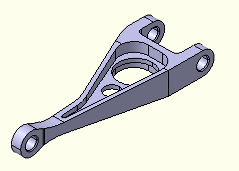
![]() This task shows you how to load the .CATPart document that contains
the model geometry for this tutorial, assign a
material to the part, and modify the material
properties.
This task shows you how to load the .CATPart document that contains
the model geometry for this tutorial, assign a
material to the part, and modify the material
properties.
-
Open the .CATPart file for this tutorial.
-
Select File>Open from the menu bar.
The File Selection dialog box appears.
-
In the File name field at the bottom of the File Selection dialog box, type install_dir\intel_a\resources\graphic\ANLDoc\sample01.CATPart, where install_dir is the name of the directory in which the Nonlinear Structural Analysis product is installed. Alternatively, you can browse to this location using the arrow next to the Look in: field and select the file from the list in the center of the dialog box.
-
Click Open in the File Selection dialog box.
The part design document is opened in the Part Design workbench, and the selected part appears in the window.
-
-
You must assign a material to a part before you can analyze it. To assign a material to the sample part, do the following:
-
Select the PartBody feature in the specification tree.
-
Click the Apply Material icon
 .
. Tip: If a toolbar
is not visible in the Nonlinear
Structural Analysis window, select
View>Toolbars>toolbar_name
from the menu bar.
Tip: If a toolbar
is not visible in the Nonlinear
Structural Analysis window, select
View>Toolbars>toolbar_name
from the menu bar.The Library dialog box opens. The default .CATMaterial document is used.
-
Select the Metal material family from the tabs along the top of the dialog box, then choose Aluminium from the displayed images, and click OK.
The material is applied to the part, and an Aluminium object appears under the PartBody objects set in the specification tree.
Note: If you enter the Nonlinear Structural Analysis workbench from a .CATPart document containing a part without a material assignment, a dialog box appears warning you that the material definition is missing. You must return to the Part Design workbench to apply a material.
-
-
To apply a render style to the part that reflects the material assignment, select View>Render Style>Customize View from the menu bar, and toggle on Material in the View Mode Customization dialog box that appears.
-
You can view and modify the material properties and analysis characteristics:
-
Click on the Aluminium object under the PartBody feature in the specification tree, and select Edit>Properties from the menu bar to edit the material properties.
The Properties dialog box appears.
-
Use the arrows near the top of the dialog box to scroll and reveal the additional tabs; click the Nonlinear and Thermal Properties tab when it appears.
A warning dialog box will appear the first time that nonlinear and thermal properties are loaded in a Nonlinear Structural Analysis session. Click OK to dismiss the warning.
-
In the list of Available Options, toggle on Elasticity.
The Elasticity option appears in the list of Selected Options on the right side of the dialog box, and the elasticity data table appears in the bottom half of the dialog box.
-
Enter a value of 7e+010 N/m2 for Young's Modulus and a value of 0.346 for Poisson's Ratio.
-
Click OK in the Properties dialog box to update the material properties for Aluminium.
-
-
Since you have made changes to the original .CATPart file, you should save it to a location where you have write permissions. Select File>Save from the menu bar, and select a directory in which you can save the file.
Creating an Analysis
Case
This task shows you to how to enter the Nonlinear Structural Analysis workbench and create an analysis case containing a general static step.
-
Select Start>Analysis & Simulation>Nonlinear Structural Analysis from the main menu bar.
The New Analysis Case dialog box appears with the default Nonlinear Structural Analysis type selected.
-
Click OK in the New Analysis Case dialog box to enter the Nonlinear Structural Analysis workbench.
 Warning: Do not select
Keep
as default starting analysis case in
the New Analysis Case dialog
box.
Warning: Do not select
Keep
as default starting analysis case in
the New Analysis Case dialog
box.A .CATAnalysis document named Analysis1 opens. A link exists between the .CATPart and the .CATAnalysis document. In addition, the standard structure of the Analysis Manager specification tree is displayed.
The Nonlinear Structural Case objects set contains a Simulation History objects set with an Initialization step and a Static Step objects set, a Jobs objects set containing a default job, and empty Display Groups and Analysis Case Solution objects sets. The Simulation History will contain a description of the environmental influences on the model, which generally vary as a function of time over a period defined by the user. (See Specification Tree for more details on the specification tree.)
-
To edit the static step created with the analysis case, double-click on the Static Step–1 objects set in the specification tree under the Simulation History objects set for the current analysis case. (The current analysis case is the one most recently created or edited; it is underlined in the specification tree.)
Nonlinear Structural Analysis opens the Static Step dialog box.
Note: To create a new static step, you can click the General Static Step icon
 .
. -
You can change the step identifier for the Static Step by editing the Step name field. This name will be used in the specification tree.
-
Enter a description for the step in the Step description field. This description will appear in the input file that is written for this analysis.
-
In this example we expect that the part will deform significantly; hence, it is appropriate to consider finite deformation effects. Specify that the solver should account for nonlinear geometric effects in the step by selecting On for Nonlinear geometry.
-
Accept the default values for the other step controls.
-
Click OK when you have finished editing the step.
The Static Step objects set contains a default Field Output Request object and empty History Output Requests, Loads, Boundary Conditions, and Fields objects sets.
Defining Boundary
Conditions
This task shows you to how to apply boundary conditions to constrain your part. You will fully constrain all degrees of freedom on two faces of the part and prescribe a vertical displacement for a third face.
-
Click the Clamp Boundary Condition icon
 .
.The Clamp Boundary Condition icon is hidden by default. The small black triangles at the base of some icons indicate the presence of hidden icons that can be revealed. Click the Displacement Boundary Condition icon
 , but do not release the
mouse button. The Clamp Boundary Condition icon
appears. Without releasing the mouse button,
drag the cursor along the set of icons until
you reach the Clamp Boundary Condition icon.
Then release the mouse button to select that
icon.
, but do not release the
mouse button. The Clamp Boundary Condition icon
appears. Without releasing the mouse button,
drag the cursor along the set of icons until
you reach the Clamp Boundary Condition icon.
Then release the mouse button to select that
icon.The Clamp BC dialog box appears, and a Clamp object appears in the specification tree under the Boundary Conditions objects set for the current step.
-
You can change the boundary condition identifier by editing the Name field.
-
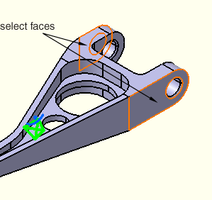
Select the two faces indicated in Figure 3–2 as supports for the boundary condition.
If necessary, reselect a face to remove it from the selection set.
The Supports field is updated to reflect your selection, and clamp symbols appear on the selected faces indicating the constrained degrees of freedom.
-
Click OK in the Clamp BC dialog box.
-
Click the Displacement Boundary Condition icon
.The Displacement BC dialog box appears, and a Displacement object appears in the specification tree under the Boundary Conditions objects set for the current step.
-
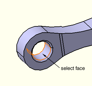
Select the face shown in Figure 3–3.
The Supports field is updated to reflect your selection, and arrows appear on the selected face indicating the constrained degrees of freedom (only the arrowheads appear for zero-valued constraints).
-
To prescribe a vertical displacement of 0.254 mm for the selected face, toggle off U1 and U2, enter a value of –0.254 mm for U3 in the Displacement BC dialog box, and click OK.
Generating a Mesh and
Submitting an Analysis Job
The finite element mesh is the collection of nodes and elements used to represent the system and to transform the continuous mechanical problem into a discrete numerical problem. All user specifications on the system geometry are eventually translated by the program into mesh input data.
![]() This task shows you how to specify mesh
parameters such as size and sag, generate the
mesh on your part, create an analysis job, and
submit the job to the solver.
This task shows you how to specify mesh
parameters such as size and sag, generate the
mesh on your part, create an analysis job, and
submit the job to the solver.
-
Expand the Nodes and Elements feature in the specification tree, and double-click the OCTREE Tetrahedron Mesh.1 feature to edit the global characteristics of the mesh.
The OCTREE Tetrahedron Mesh dialog box appears.
The important element characteristics are their order, their size, and their sag. The order is the degree of polynomial interpolation for the unknown field (the displacement field) inside the element. The size is the dimension of the element. The sag is a measure of how closely the element boundaries follow the geometry they are supposed to represent.
-
In the OCTREE Tetrahedron Mesh dialog box, specify a global element Size of 0.025 m and a global element Absolute sag of 0.008 m. Accept the default choice of a linear element type, and click OK.
-
Right-click on the Nodes and Elements object in the specification tree, and select Mesh Visualization from the menu that appears.
A warning message dialog box appears, informing you that the mesh needs to be updated; click OK to close the dialog box and continue with the mesh generation. When the mesh generation is complete, the mesh is displayed on the part and a Mesh object appears under Nodes and Elements in the specification tree.
-
Expand the Jobs object set in the specification tree, and double-click the Job-1 feature to edit the analysis job.
The Edit Job dialog box appears.
Note: To create a new job for the current analysis case, click the Create Job icon
 .
. -
You can change the job identifier by editing the Name field. This name will be used in the specification tree and in the Job Manager.
-
Enter a description for the job in the Description field.
-
Accept the default values for the job data, and click OK.
-
Save the .CATAnalysis file to a location where you have write permissions. Select File>Save from the menu bar, and select a directory in which you can save the file.
-
Click the Job Manager icon
 .
.The Job Manager dialog box appears with a list of the jobs that you have created. By default, jobs for all Analysis Cases are shown.
-
Select the job you edited from the list in the Job Manager, and click Submit.
By default, consistency checks are run when a job is submitted. A Job Submission dialog box appears with the results of these consistency checks. In addition to the consistency check messages, messages from the input file writer are listed on the Write Input File Messages tabbed page. In this case the Consistency Check Messages page is empty, and the Write Input File Messages page indicates that the input file was generated successfully.
-
Click Continue in the Job Submission dialog box.
Nonlinear Structural Analysis submits the job for analysis using the job settings defined in the job editor. The information in the Status column of the Job Manager updates to indicate the job's status. The Status column for this tutorial shows one of the following:
-
Submitted while the analysis input file is being generated.
-
Running while the solver analyzes the model.
-
Completed when the analysis is complete, and the output has been written to the output database file.
-
Aborted if the solver finds a problem with the input file or the analysis and aborts the analysis.
-
-
When the job completes successfully, you are ready to review the results of the analysis. From the buttons on the right edge of the Job Manager, click Attach Results.
A link to the output database file containing the results appears in the Links Manager, and a Static Step object appears in the specification tree under the Analysis Case Solution objects set for the current analysis case. In addition, the status of the Analysis Case Solution entry is updated to show that the solution is now available and is consistent with the model and history specification; in other words, the
 symbol
no longer appears.
symbol
no longer appears. -
Click Close in the Job Manager.
Viewing Stress
Results
This task shows you how to visualize results from your analysis.
-
Right-click on the Static Step object under the Analysis Case Solution objects set in the specification tree, and select Generate Results Image from the menu that appears.
Alternatively, you can select the Static Step object in the specification tree to make it active and click the Generate Results Image icon
 .
.The Abaqus Image Generation dialog box appears with a list of the results available from the output database file for the specified step.
-
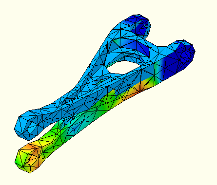
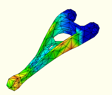
To plot contour values of the nodal von Mises stresses in your model, select Von Mises Stress from the list of Available Images, and click OK.
The Abaqus Image Generation dialog box disappears, and the von Mises stress is plotted on the deformed shape of the model, as shown in Figure 3–4. A feature for the generated image appears under the Static Step object in the specification tree.
-
To remove the undeformed shape of the model from the display, right-click on the Nodes and Elements feature in the specification tree and select Hide/Show from the menu that appears.
The undeformed shape disappears from view; you can clearly see the von Mises stress contours, as shown in Figure 3–5.
-
To view an animation of the von Mises stresses, click the Animate icon
 in the Analysis
Tools toolbar.
in the Analysis
Tools toolbar.The Animate dialog box appears, and the von Mises stress image is animated in the main window with the default animation parameters. By default, an animated image of the stresses is created by stepping through every increment in the analysis.
-
To animate the stresses by applying a scale factor to the stress values in the current analysis step, perform the following steps:
-
Click the Amplification Magnitude icon
 in
the Analysis Tools toolbar.
in
the Analysis Tools toolbar.The Amplification Magnitude dialog box appears.
-
If the Scaling factor option is not selected, toggle it on.
-
Change the scaling factor for the animation by dragging the slider or by specifying a new value in the Factor field, then click OK.
Your scaling changes will take effect upon a restart of the animation.
-
-
Click Close in the Animate dialog box to stop the animation.
You have now finished the tutorial.
For information on related topics, click the following item: