This task shows you how to load the .CATPart document that contains the model geometry for this tutorial and how to add temperature-dependent material properties to the material definition.

1. Open the .CATPart file for this tutorial.

   1. Select File>Open from the menu bar.

      The File Selection dialog box appears.

   2. In the File name field at the bottom of the File Selection dialog box, type install_dir\intel_a\resources\graphic\ANLDoc\sample02.CATPart, where install_dir is the name of the directory in which the Thermal Analysis product is installed. Alternatively, you can browse to this location using the arrow next to the Look in: field and select the file from the list in the center of the dialog box.

   3. Click Open in the File Selection dialog box.

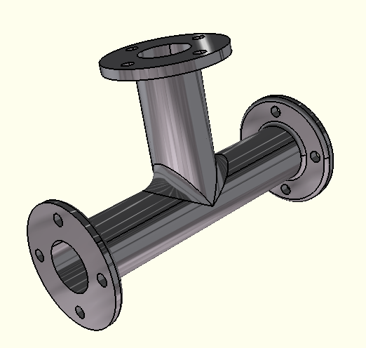
   The part design document is opened in the Part Design workbench, and the selected part appears in the window, as shown in Figure 3–6.

   Figure 3–6 The sample02.CATPart model.

   

2. Modify the material properties.

   1. Click on the Aluminium object under the PartBody feature in the specification tree, and select Edit>Properties from the menu bar to edit the material properties.

      The Properties dialog box appears.

   2. Use the arrows near the top of the dialog box to scroll and reveal additional tabs; click the Nonlinear and Thermal Properties tab when it appears.

      A warning dialog box will appear the first time that nonlinear and thermal properties are loaded in a Thermal Analysis session. Click OK to dismiss the warning.

   3. In the list of Available Options, toggle on Elasticity; enter a value of 6.9E10 N/m² for Young’s Modulus and a value of 0.33 for Poisson’s Ratio.

   4. Toggle on Plasticity. Under the Plasticity field, toggle on Use temperature-dependent data. Click the Import data from file icon at the bottom of the Properties dialog box. In the File name field at the bottom of the Open File dialog box that appears, type install_dir\intel_a\resources\graphic\ANLDoc\plasticProps.txt, where install_dir is the name of the directory in which Thermal Analysis is installed, and click Open.

      The stress/strain data are imported into the Plasticity table.

   5. Toggle on Density, and enter a value of 2700 kg/m³.

   6. Toggle on Thermal Conductivity. Under the Thermal Conductivity field, toggle on Use temperature-dependent data. Enter a value of 204 W/mK for a temperature of 273 K. Click Add to add a row to the table, and enter a value of 225 W/mK for a temperature of 573 K.

   7. Toggle on Specific Heat, and enter a value of 0.88 KJ/kgK.

   8. Toggle on Coefficient of Thermal Expansion, and enter a value of 8.42E–5/K.

   9. Click OK in the Properties dialog box to update the material properties.

3. Since you have made changes to the original .CATPart file, you should save it to a location where you have write permissions. Select File>Save from the menu bar, and select a directory in which you can save the file.

1. Select Start>Analysis & Simulation>Thermal Analysis from the main menu bar.

   The New Analysis Case dialog box appears with the default Thermal Analysis type selected.

2. Click OK in the New Analysis Case dialog box to enter the Thermal Analysis workbench.

   Warning:  Do not select Keep as default starting analysis case in the New Analysis Case dialog box.

   A .CATAnalysis document named Analysis1 opens. A link exists between the .CATPart and the .CATAnalysis document. In addition, the standard structure of the Analysis Manager specification tree is displayed.

   The Thermal Case objects set contains a Simulation History objects set with an Initialization step and a Heat Transfer Step objects set, a Jobs objects set containing a default job, and empty Display Groups and Analysis Case Solution objects sets. The Simulation History will contain a description of the environmental influences on the model, which generally vary as a function of time over a period defined by the user. (See Specification Tree for more details on the specification tree.)

3. To edit the heat transfer step created with the analysis case, double-click on the Heat Transfer Step–1 objects set in the specification tree under the Simulation History objects set for the current analysis case. (The current analysis case is the one most recently created or edited; it is underlined in the specification tree.)

   The Thermal Analysis workbench opens the Heat Transfer Step dialog box.

   Note:  To create a new heat transfer step, you can click the Heat Transfer Step icon .

4. You can change the step identifier by editing the Step name field. This name will be used in the specification tree.

5. Enter Computation of temperature distribution as the Step description. This description will appear in the input file that is written for this analysis.

6. Modify the Basic Step Data:

   1. Enter a value of 200 seconds for the Step time.

   2. Enter a value of 1 second for the Initial increment size.

   3. Enter a value of 10 seconds for the Maximum increment size.

7. Modify the Heat Transfer Data:

   1. Toggle on Transient as the Thermal response.

   2. Toggle on End step when temperature change rate is less than, and enter a value of 0.5 Kdeg for this option.

   3. Enter a value of 10 Kdeg for the Maximum temperature change allowed per increment.

8. Click OK when you have finished editing the step.

   The Heat Transfer Step objects set contains a default Field Output Request object in a Field Output Request objects set and empty History Output Requests, Loads, and Boundary Conditions objects sets.

9. When defining a film condition, you must select all of the faces on the model to which the film condition applies. Defining surface groups simplifies the process of defining a film condition. A group is a preselected set of geometric entities that can be used as a support for model property definitions. Groups are saved in the specification tree and can be reused in multiple property definitions.

   1. Click the Surface Group icon .

      The Surface Group dialog box appears, and a Surface Group object appears in the specification tree under the Groups objects set.

   2. Enter OuterSurface in the Name field. This name appears in the specification tree as the identifier for the group.

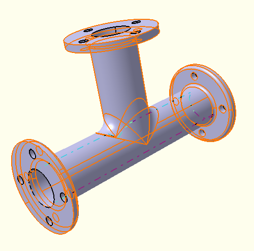
   3. Select the 25 faces constituting the outer surface of the pipe, as shown in Figure 3–7.

      Figure 3–7 Select the highlighted faces to define the OuterSurface group.

      

      Tip: It is easier to manipulate the model if the render style is set to Shading with Edges. From the main menu bar, select View>Render Style>Shading with Edges. Reselect a face to deselect it if necessary. There should be 7 faces on each of the left and right flanges, 5 faces on the top flange, and 6 faces on the main T-shaped cylinder.

   4. Click OK when you have finished selecting the faces.

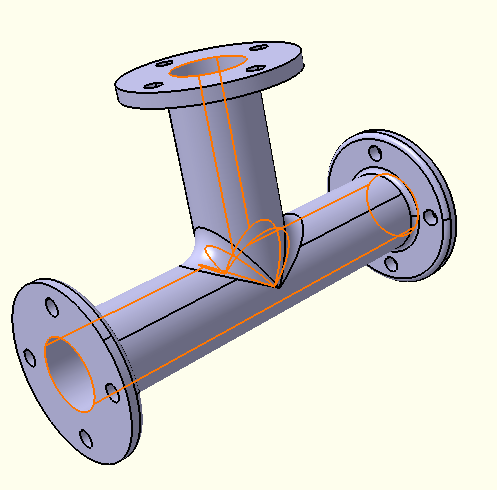
   5. Repeat the above steps to create another group called InnerSurface that consists of the inner faces of the pipe. The inner surface is shown in Figure 3–8; it is composed of 6 faces.

      Figure 3–8 Select the highlighted faces to define the InnerSurface group.

      

10. Define the film conditions.

    1. Click the Film Condition icon .

       The Film Condition dialog box appears.

    2. You can change the identifier of the load by editing the Name field.

    3. Select the OuterSurface group in the specification tree as the support for the load.

       1 Face appears in the Support field to reflect your selection; however, the load will be applied to all 25 faces that are part of the OuterSurface group definition.

    4. By default, the film coefficient is assumed to be a function of surface temperature. In this example the film coefficient is constant; therefore, toggle off Use temperature-dependent data, and enter a value of 50 W/m²K for the film coefficient.

    5. Enter a value of 293 Kdeg for the Reference sink temperature.

    6. Click OK in the Film Condition dialog box.

       A Film Condition object appears in the specification tree under the Loads objects set for the current step, and symbols indicating the applied film condition are displayed on the selected faces.

    7. Repeat the above steps to define the film condition for the inner surface of the pipe, using the InnerSurface group as the support, a film coefficient of 1200 W/m²K, and a reference sink temperature of 673 Kdeg.

11. Define the initial conditions.

    1. Click the Initial Temperature icon .

       The Initial Temperature dialog box appears.

    2. You can change the identifier of the field by editing the Name field.

    3. Select the PartBody feature in the specification tree to apply the initial temperature to the entire model.

       The entire part is highlighted, and the Supports field is updated to reflect your selection.

    4. Use the default Uniform distribution type, and enter a value of 293 Kdeg for the Magnitude of the initial temperature.

    5. Click OK in the Initial Temperature dialog box.

       An Initial Temperature object appears in the specification tree under the Fields objects set in the Initialization step, and symbols indicating the applied temperature are displayed on the entire model.

1. Expand the Nodes and Elements feature in the specification tree, and double-click the OCTREE Tetrahedron Mesh.1 feature to edit the global characteristics of the mesh.

   The OCTREE Tetrahedron Mesh dialog box appears.

2. In the OCTREE Tetrahedron Mesh dialog box, specify a global element Size of 0.05 m and a global element Absolute sag of 0.015 m. Accept the default choice of a linear element type, and click OK.

3. Right-click on the Nodes and Elements object in the specification tree, and select Mesh Visualization from the menu that appears.

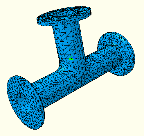
   A warning message dialog box appears, informing you that the mesh needs to be updated; click OK to close the dialog box and to continue with the mesh generation. When the mesh generation is complete, the mesh is displayed on the part (see Figure 3–9) and a Mesh object appears under Nodes and Elements in the specification tree.

   Figure 3–9 The meshed pipe model.

   

4. Expand the Jobs object set in the specification tree, and double-click the Job–1 feature to edit the analysis job.

   The Edit Job dialog box appears.

   Note:  To create a new job for the current analysis case, click the Create Job icon .

5. You can change the job identifier by editing the Name field. This name will be used in the specification tree and in the Job Manager.

6. Enter a description for the job in the Description field.

7. Accept the default values for the job data, and click OK.

8. Click the Job Manager icon .

   The Job Manager dialog box appears with a list of the jobs that you have created. By default, jobs for all Nonlinear and Thermal Analysis Cases are shown.

9. Select the job you created from the list in the Job Manager, and click Submit.

   By default, consistency checks are run when you submit a job. A Job Submission dialog box appears with the results of the consistency checks:

   
   
   

   Feature Name	Feature Type	Message	Severity
   Boundary Conditions/Heat Transfer Step-1	Boundary Condition Set	Boundary condition set is empty	Warning

   
   
   

10. Click Continue.

    Thermal Analysis submits the job for analysis using the job settings defined in the job editor. The information in the Status column of the Job Manager updates to indicate the job's status. The Status column for this tutorial shows one of the following:

    • Submitted while the analysis input file is being generated.

    • Running while the solver analyzes the model.

    • Completed when the analysis is complete, and the output has been written to the output database file.

    • Aborted if the solver finds a problem with the input file or the analysis and aborts the analysis.

11. While the job is running, click Monitor in the Job Manager to monitor the progress of the analysis.

    The job monitor dialog box appears. The top half of the dialog box displays the information available in the status (.sta) file that the solver creates for the job. The bottom half of the dialog box displays log file information, error and warning messages, and output information.

12. When the job completes successfully, click Close in the Job Monitor dialog box, and click Attach Results in the Job Manager.

    A link to the output database file containing the results appears in the Links Manager, and a Heat Transfer Step object appears in the specification tree under the Analysis Case Solution objects set for the current analysis case. In addition, the status of the Analysis Case Solution entry is updated to show that the solution is now available and is consistent with the model and history specification; in other words, the symbol no longer appears.

13. Plot the nodal temperatures.

    1. Right-click on the Heat Transfer Step object under the Analysis Case Solution objects set in the specification tree, and select Generate Results Image from the menu that appears.

       The Abaqus Image Generation dialog box appears with a list of the results available from the output database file for the specified step.

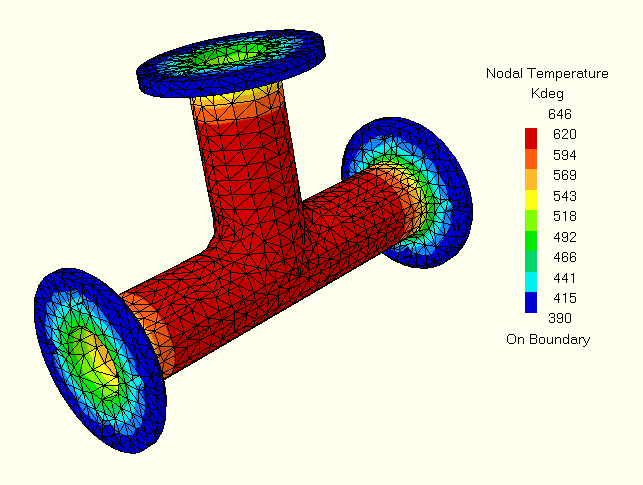
    2. To plot contour values of nodal temperature for your model, select Nodal Temperature from the list of Available Images, and click OK.

       The Abaqus Image Generation dialog box disappears, and the nodal temperatures are plotted on the model, as shown in Figure 3–10. A feature for the generated image appears under the Heat Transfer Step object in the specification tree.

       Figure 3–10 Contour plot of nodal temperatures.

       

       You may need to hide the nodes and elements and change the render style to view the contour plot clearly. Right-click on the Nodes and Elements feature in the specification tree, and select Hide/Show from the menu that appears. To apply a render style to the part that reflects the material assignment, select View>Render Style>Customize View from the menu bar, and toggle on Materials in the Custom View Modes dialog box that appears.

1. Switch to the Nonlinear Structural Analysis workbench by selecting Start>Analysis and Simulation>Nonlinear Structural Analysis from the main menu bar.

2. Select Insert>Nonlinear Structural Case from the menu bar.

   Nonlinear Structural-Case-1 is created and appended to the specification tree.

   Note:  Nonlinear Structural-Case-1 is underlined in the specification tree, which indicates that it is now the current analysis case. This case will be modified when you add or edit step definitions, and it will be used for analysis submission. You can make an analysis case current by right-clicking on it and selecting Set As Current Case from the menu that appears.

3. Click the Pressure Load icon to add a pressure load to the current step. Select the six internal surfaces shown in Figure 3–8. In the Pressure dialog box, enter a value of 3.5E06 N/m² for the pressure, and click OK.

   Symbols representing the applied pressure are displayed on the geometry, and a Pressure object appears in the specification tree under the Loads objects set for the current step—the general static step in the new structural case.

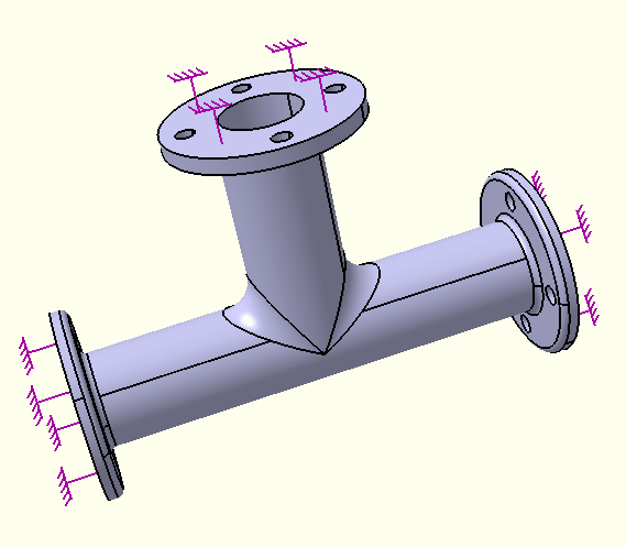
4. Click the Clamp Boundary Condition icon . Select the three flange faces shown in Figure 3–11 and click OK in the Clamp BC dialog box.

   Figure 3–11 Apply a clamp boundary condition to the three flange faces.

   

   A Clamp object appears in the specification tree under the Boundary Conditions objects set for the current step, and symbols appear on the selected faces indicating the constrained degrees of freedom.

5. Click the General Static Step icon to create a second step. In the General Static Step dialog box, enter a value of 200 seconds for the Step time, 20 seconds for the Initial increment size, and 200 seconds for the Maximum increment size. Accept the other default values, and click OK.

   A second Static Step objects set appears in the specification tree under the Simulation History objects set for the current analysis case.

   Note:  The Static Step-2 object in the specification tree is now underlined, indicating that for the current analysis case, this is the step for which you are now defining loads and boundary conditions.

6. Click the Temperature History icon . Select the entire part by selecting the PartBody feature from the specification tree. In the Temperature History dialog box, select From job as the Distribution Type. Then select Job-1 in Thermal-Case-1 from the specification tree to identify the job from which the results should be read, and click OK.

   Symbols representing the applied field are displayed on the geometry, and a Temperature History object appears in the specification tree under the Fields objects set for the current step.

7. Double-click the Job–2 feature located in the Jobs object set for Nonlinear Structural-Case-1 in the specification tree.

   The Edit Job dialog box appears.

8. Enter a name and description for the job, accept the default values for the job data, and click OK.

9. Click the Job Manager icon , select the new job from the list in the Job Manager, and click Submit.

10. Click Continue in the Job Submission dialog box that appears with a list of informational consistency check messages.

11. When the analysis completes, click Attach Results in the Job Manager, and click OK in the dialog box that appears.

    A link to the output database file containing the results appears in the Links Manager, and two Static Step objects (one for each step) appear in the specification tree under the Analysis Case Solution feature.

1. For each step:

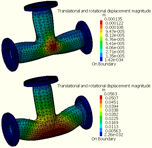
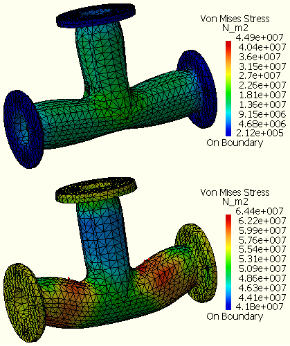
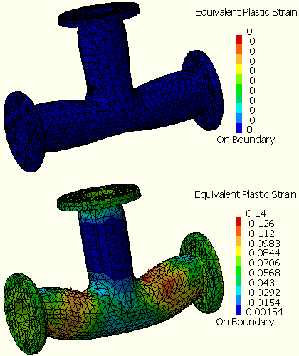
   1. Right-click on the Static Step object under the Analysis Case Solution objects set in the specification tree, and select Generate Results Image from the menu that appears.

   2. Successively select Translational and rotational displacement magnitude, Von Mises Stress, and Equivalent Plastic Strain from the list of Available Images and click OK to create the contour plots shown in Figure 3–12 Figure 3–13 and Figure 3–14.

      By default, the previous image is deactivated from the display when you create a new contour plot image. To view a previously created image, right-click on the image name in the specification tree, and select Activate/Deactivate from the menu that appears. Use the same procedure to deactivate the current image if necessary.

      Figure 3–12 Contour plots of displacement for Step 1 (top) and Step 2 (bottom).

      

      Figure 3–13 Contour plots of von Mises stress for Step 1 (top) and Step 2 (bottom).

      

      Figure 3–14 Contour plots of equivalent plastic strain for Step 1 (top) and Step 2 (bottom).

      

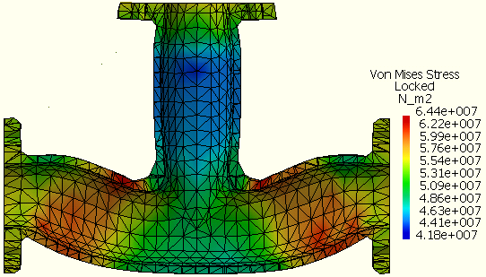
2. Perform a cut plane analysis.

   1. Click the Cut Plane Analysis icon .

      The cutting plane appears in the main window; in addition, the Cut Plane Analysis dialog box appears. The compass is positioned automatically on the model, and the cutting plane is positioned normal to the privileged direction of the compass.

      Note:  If the compass is already positioned in the view, the normal of the compass is considered to be the default normal of the cutting plane.

   2. Rotate the cutting plane by clicking on the circular arcs of the compass and dragging the cursor; translate the cutting plane by clicking on the straight edges of the compass and dragging the cursor. Orient the cutting plane so that it cuts the pipe intersection in a plane parallel to the pipe axes, as shown in Figure 3–15.

      Figure 3–15 Cut plane view of the pipe model.

      

      As you modify the position of the plane, the results in the plane are updated automatically.